This is the multi-page printable view of this section. Click here to print.
Kafka Streams
1 - Introduction
Streams
Overview
Kafka Streams is a client library for processing and analyzing data stored in Kafka and either write the resulting data back to Kafka or send the final output to an external system. It builds upon important stream processing concepts such as properly distinguishing between event time and processing time, windowing support, and simple yet efficient management of application state.
Kafka Streams has a low barrier to entry : You can quickly write and run a small-scale proof-of-concept on a single machine; and you only need to run additional instances of your application on multiple machines to scale up to high-volume production workloads. Kafka Streams transparently handles the load balancing of multiple instances of the same application by leveraging Kafka’s parallelism model.
Some highlights of Kafka Streams:
- Designed as a simple and lightweight client library , which can be easily embedded in any Java application and integrated with any existing packaging, deployment and operational tools that users have for their streaming applications.
- Has no external dependencies on systems other than Apache Kafka itself as the internal messaging layer; notably, it uses Kafka’s partitioning model to horizontally scale processing while maintaining strong ordering guarantees.
- Supports fault-tolerant local state , which enables very fast and efficient stateful operations like windowed joins and aggregations.
- Employs one-record-at-a-time processing to achieve millisecond processing latency, and supports event-time based windowing operations with late arrival of records.
- Offers necessary stream processing primitives, along with a high-level Streams DSL and a low-level Processor API.
Previous Next
2 - Core Concepts
Core Concepts
We first summarize the key concepts of Kafka Streams.
Stream Processing Topology
- A stream is the most important abstraction provided by Kafka Streams: it represents an unbounded, continuously updating data set. A stream is an ordered, replayable, and fault-tolerant sequence of immutable data records, where a data record is defined as a key-value pair.
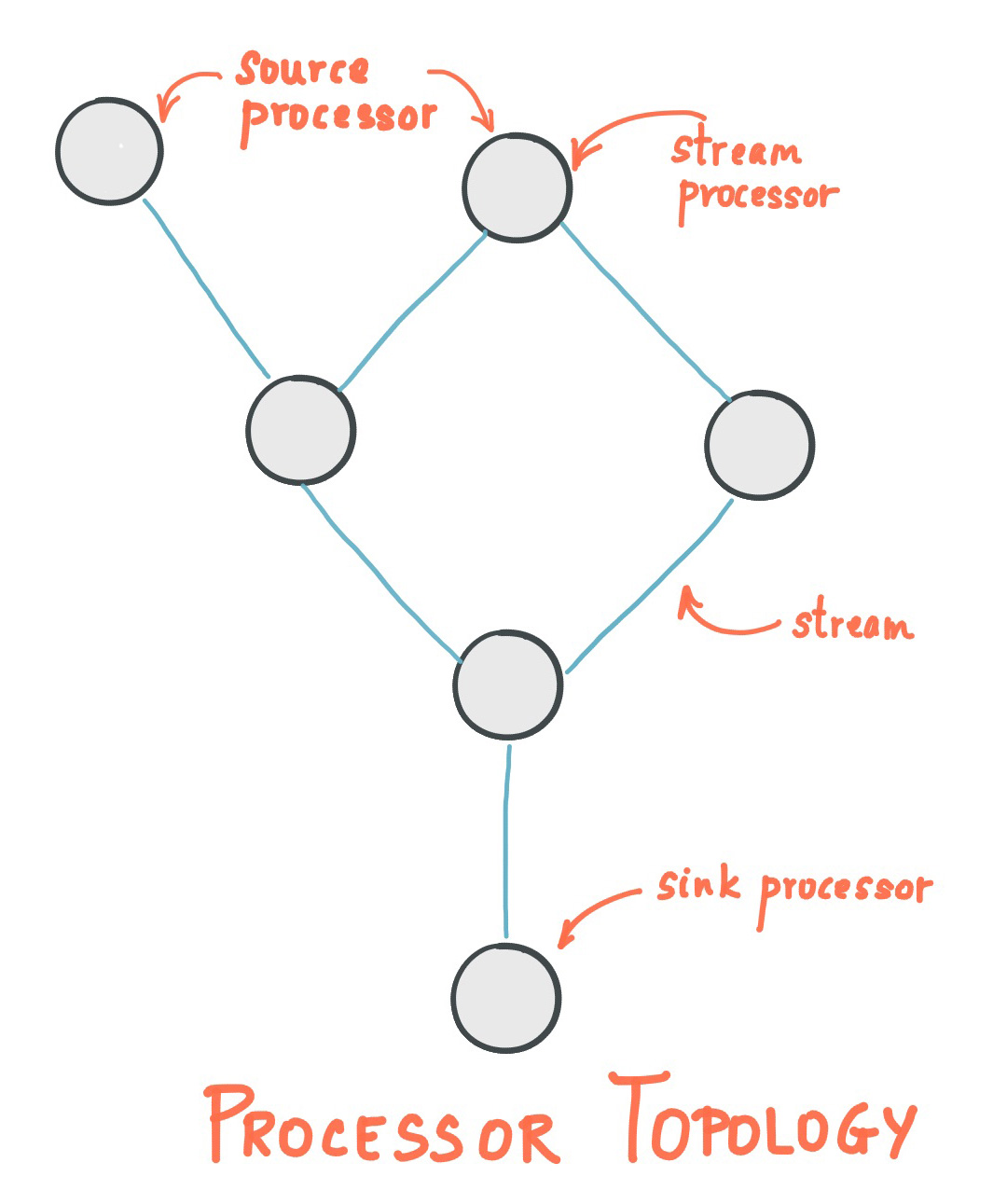
- A stream processing application is any program that makes use of the Kafka Streams library. It defines its computational logic through one or more processor topologies , where a processor topology is a graph of stream processors (nodes) that are connected by streams (edges).
- A stream processor is a node in the processor topology; it represents a processing step to transform data in streams by receiving one input record at a time from its upstream processors in the topology, applying its operation to it, and may subsequently produce one or more output records to its downstream processors.
There are two special processors in the topology:
- Source Processor : A source processor is a special type of stream processor that does not have any upstream processors. It produces an input stream to its topology from one or multiple Kafka topics by consuming records from these topics and forward them to its down-stream processors.
- Sink Processor : A sink processor is a special type of stream processor that does not have down-stream processors. It sends any received records from its up-stream processors to a specified Kafka topic.
Kafka Streams offers two ways to define the stream processing topology: the Kafka Streams DSL provides the most common data transformation operations such as map, filter, join and aggregations out of the box; the lower-level Processor API allows developers define and connect custom processors as well as to interact with state stores.
A processor topology is merely a logical abstraction for your stream processing code. At runtime, the logical topology is instantiated and replicated inside the application for parallel processing (see Stream Partitions and Tasks for details).
Time
A critical aspect in stream processing is the notion of time , and how it is modeled and integrated. For example, some operations such as windowing are defined based on time boundaries.
Common notions of time in streams are:
- Event time - The point in time when an event or data record occurred, i.e. was originally created “at the source”. Example: If the event is a geo-location change reported by a GPS sensor in a car, then the associated event-time would be the time when the GPS sensor captured the location change.
- Processing time - The point in time when the event or data record happens to be processed by the stream processing application, i.e. when the record is being consumed. The processing time may be milliseconds, hours, or days etc. later than the original event time. Example: Imagine an analytics application that reads and processes the geo-location data reported from car sensors to present it to a fleet management dashboard. Here, processing-time in the analytics application might be milliseconds or seconds (e.g. for real-time pipelines based on Apache Kafka and Kafka Streams) or hours (e.g. for batch pipelines based on Apache Hadoop or Apache Spark) after event-time.
- Ingestion time - The point in time when an event or data record is stored in a topic partition by a Kafka broker. The difference to event time is that this ingestion timestamp is generated when the record is appended to the target topic by the Kafka broker, not when the record is created “at the source”. The difference to processing time is that processing time is when the stream processing application processes the record. For example, if a record is never processed, there is no notion of processing time for it, but it still has an ingestion time.
The choice between event-time and ingestion-time is actually done through the configuration of Kafka (not Kafka Streams): From Kafka 0.10.x onwards, timestamps are automatically embedded into Kafka messages. Depending on Kafka’s configuration these timestamps represent event-time or ingestion-time. The respective Kafka configuration setting can be specified on the broker level or per topic. The default timestamp extractor in Kafka Streams will retrieve these embedded timestamps as-is. Hence, the effective time semantics of your application depend on the effective Kafka configuration for these embedded timestamps.
Kafka Streams assigns a timestamp to every data record via the TimestampExtractor interface. Concrete implementations of this interface may retrieve or compute timestamps based on the actual contents of data records such as an embedded timestamp field to provide event-time semantics, or use any other approach such as returning the current wall-clock time at the time of processing, thereby yielding processing-time semantics to stream processing applications. Developers can thus enforce different notions of time depending on their business needs. For example, per-record timestamps describe the progress of a stream with regards to time (although records may be out-of-order within the stream) and are leveraged by time-dependent operations such as joins.
Finally, whenever a Kafka Streams application writes records to Kafka, then it will also assign timestamps to these new records. The way the timestamps are assigned depends on the context:
- When new output records are generated via processing some input record, for example,
context.forward()triggered in theprocess()function call, output record timestamps are inherited from input record timestamps directly. - When new output records are generated via periodic functions such as
punctuate(), the output record timestamp is defined as the current internal time (obtained throughcontext.timestamp()) of the stream task. - For aggregations, the timestamp of a resulting aggregate update record will be that of the latest arrived input record that triggered the update.
States
Some stream processing applications don’t require state, which means the processing of a message is independent from the processing of all other messages. However, being able to maintain state opens up many possibilities for sophisticated stream processing applications: you can join input streams, or group and aggregate data records. Many such stateful operators are provided by the Kafka Streams DSL.
Kafka Streams provides so-called state stores , which can be used by stream processing applications to store and query data. This is an important capability when implementing stateful operations. Every task in Kafka Streams embeds one or more state stores that can be accessed via APIs to store and query data required for processing. These state stores can either be a persistent key-value store, an in-memory hashmap, or another convenient data structure. Kafka Streams offers fault-tolerance and automatic recovery for local state stores.
Kafka Streams allows direct read-only queries of the state stores by methods, threads, processes or applications external to the stream processing application that created the state stores. This is provided through a feature called Interactive Queries. All stores are named and Interactive Queries exposes only the read operations of the underlying implementation.
3 - Architecture
Architecture
Kafka Streams simplifies application development by building on the Kafka producer and consumer libraries and leveraging the native capabilities of Kafka to offer data parallelism, distributed coordination, fault tolerance, and operational simplicity. In this section, we describe how Kafka Streams works underneath the covers.
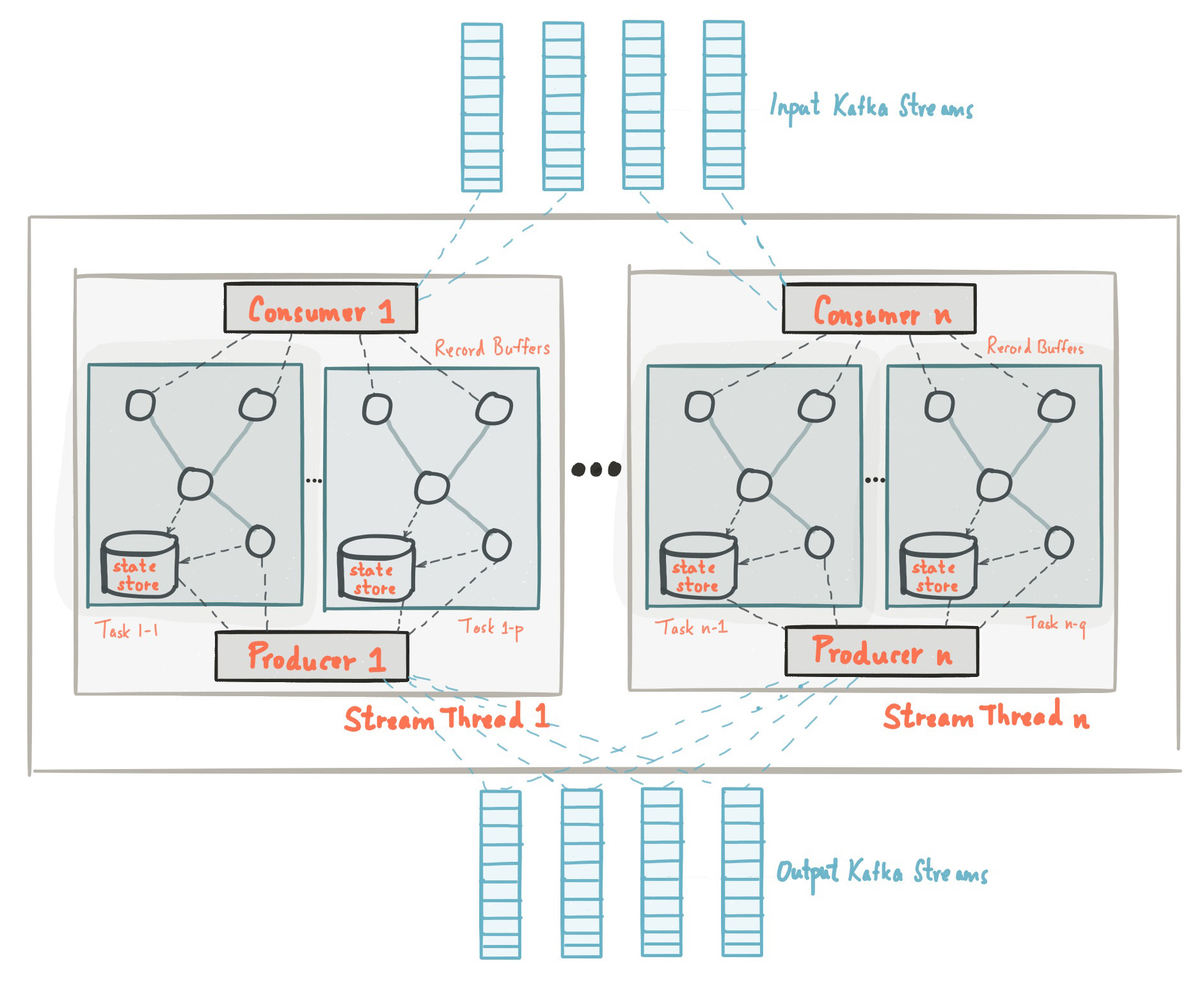
The picture below shows the anatomy of an application that uses the Kafka Streams library. Let’s walk through some details.
Stream Partitions and Tasks
The messaging layer of Kafka partitions data for storing and transporting it. Kafka Streams partitions data for processing it. In both cases, this partitioning is what enables data locality, elasticity, scalability, high performance, and fault tolerance. Kafka Streams uses the concepts of partitions and tasks as logical units of its parallelism model based on Kafka topic partitions. There are close links between Kafka Streams and Kafka in the context of parallelism:
- Each stream partition is a totally ordered sequence of data records and maps to a Kafka topic partition.
- A data record in the stream maps to a Kafka message from that topic.
- The keys of data records determine the partitioning of data in both Kafka and Kafka Streams, i.e., how data is routed to specific partitions within topics.
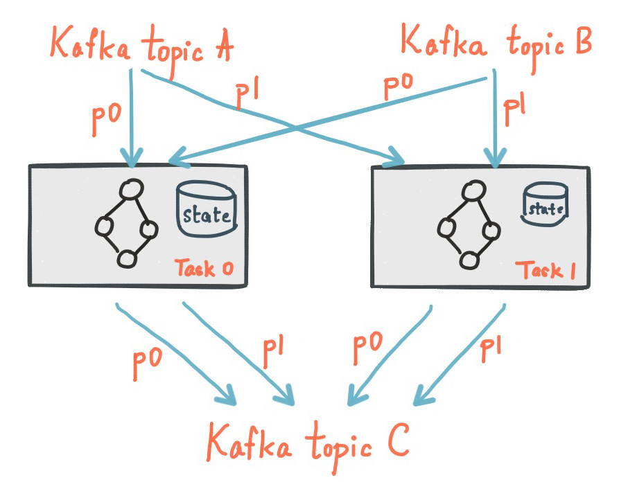
An application’s processor topology is scaled by breaking it into multiple tasks. More specifically, Kafka Streams creates a fixed number of tasks based on the input stream partitions for the application, with each task assigned a list of partitions from the input streams (i.e., Kafka topics). The assignment of partitions to tasks never changes so that each task is a fixed unit of parallelism of the application. Tasks can then instantiate their own processor topology based on the assigned partitions; they also maintain a buffer for each of its assigned partitions and process messages one-at-a-time from these record buffers. As a result stream tasks can be processed independently and in parallel without manual intervention.
Slightly simplified, the maximum parallelism at which your application may run is bounded by the maximum number of stream tasks, which itself is determined by maximum number of partitions of the input topic(s) the application is reading from. For example, if your input topic has 5 partitions, then you can run up to 5 applications instances. These instances will collaboratively process the topic’s data. If you run a larger number of app instances than partitions of the input topic, the “excess” app instances will launch but remain idle; however, if one of the busy instances goes down, one of the idle instances will resume the former’s work.
It is important to understand that Kafka Streams is not a resource manager, but a library that “runs” anywhere its stream processing application runs. Multiple instances of the application are executed either on the same machine, or spread across multiple machines and tasks can be distributed automatically by the library to those running application instances. The assignment of partitions to tasks never changes; if an application instance fails, all its assigned tasks will be automatically restarted on other instances and continue to consume from the same stream partitions.
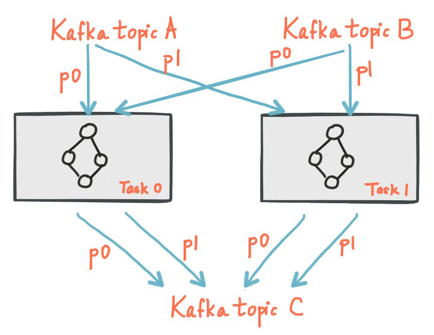
The following diagram shows two tasks each assigned with one partition of the input streams.
Threading Model
Kafka Streams allows the user to configure the number of threads that the library can use to parallelize processing within an application instance. Each thread can execute one or more tasks with their processor topologies independently. For example, the following diagram shows one stream thread running two stream tasks.
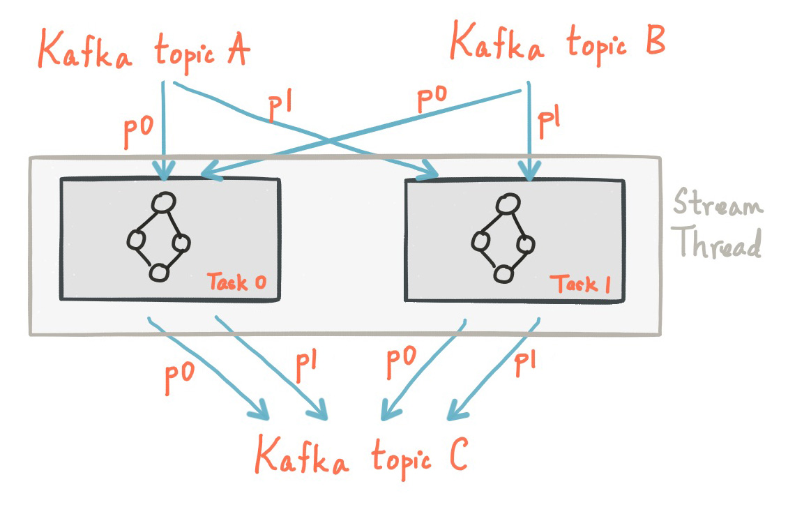
Starting more stream threads or more instances of the application merely amounts to replicating the topology and having it process a different subset of Kafka partitions, effectively parallelizing processing. It is worth noting that there is no shared state amongst the threads, so no inter-thread coordination is necessary. This makes it very simple to run topologies in parallel across the application instances and threads. The assignment of Kafka topic partitions amongst the various stream threads is transparently handled by Kafka Streams leveraging Kafka’s coordination functionality.
As we described above, scaling your stream processing application with Kafka Streams is easy: you merely need to start additional instances of your application, and Kafka Streams takes care of distributing partitions amongst tasks that run in the application instances. You can start as many threads of the application as there are input Kafka topic partitions so that, across all running instances of an application, every thread (or rather, the tasks it runs) has at least one input partition to process.
Local State Stores
Kafka Streams provides so-called state stores , which can be used by stream processing applications to store and query data, which is an important capability when implementing stateful operations. The Kafka Streams DSL, for example, automatically creates and manages such state stores when you are calling stateful operators such as join() or aggregate(), or when you are windowing a stream.
Every stream task in a Kafka Streams application may embed one or more local state stores that can be accessed via APIs to store and query data required for processing. Kafka Streams offers fault-tolerance and automatic recovery for such local state stores.
The following diagram shows two stream tasks with their dedicated local state stores.
Fault Tolerance
Kafka Streams builds on fault-tolerance capabilities integrated natively within Kafka. Kafka partitions are highly available and replicated; so when stream data is persisted to Kafka it is available even if the application fails and needs to re-process it. Tasks in Kafka Streams leverage the fault-tolerance capability offered by the Kafka consumer client to handle failures. If a task runs on a machine that fails, Kafka Streams automatically restarts the task in one of the remaining running instances of the application.
In addition, Kafka Streams makes sure that the local state stores are robust to failures, too. For each state store, it maintains a replicated changelog Kafka topic in which it tracks any state updates. These changelog topics are partitioned as well so that each local state store instance, and hence the task accessing the store, has its own dedicated changelog topic partition. Log compaction is enabled on the changelog topics so that old data can be purged safely to prevent the topics from growing indefinitely. If tasks run on a machine that fails and are restarted on another machine, Kafka Streams guarantees to restore their associated state stores to the content before the failure by replaying the corresponding changelog topics prior to resuming the processing on the newly started tasks. As a result, failure handling is completely transparent to the end user.
Note that the cost of task (re)initialization typically depends primarily on the time for restoring the state by replaying the state stores’ associated changelog topics. To minimize this restoration time, users can configure their applications to have standby replicas of local states (i.e. fully replicated copies of the state). When a task migration happens, Kafka Streams then attempts to assign a task to an application instance where such a standby replica already exists in order to minimize the task (re)initialization cost. See num.standby.replicas at the Kafka Streams Configs Section.
4 - Upgrade Guide
Upgrade Guide & API Changes
If you want to upgrade from 0.10.1.x to 0.10.2, see the Upgrade Section for 0.10.2. It highlights incompatible changes you need to consider to upgrade your code and application. See below a complete list of 0.10.2 API and semantical changes that allow you to advance your application and/or simplify your code base, including the usage of new features.
If you want to upgrade from 0.10.0.x to 0.10.1, see the Upgrade Section for 0.10.1. It highlights incompatible changes you need to consider to upgrade your code and application. See below a complete list of 0.10.1 API changes that allow you to advance your application and/or simplify your code base, including the usage of new features.
Notable changes in 0.10.2.1
Parameter updates in StreamsConfig:
- of particular importance to improve the resiliency of a Kafka Streams application are two changes to default parameters of producer
retriesand consumermax.poll.interval.ms
Streams API changes in 0.10.2.0
New methods in KafkaStreams:
- set a listener to react on application state change via
#setStateListener(StateListener listener) - retrieve the current application state via
#state() - retrieve the global metrics registry via
#metrics() - apply a timeout when closing an application via
#close(long timeout, TimeUnit timeUnit) - specify a custom indent when retrieving Kafka Streams information via
#toString(String indent)
Parameter updates in StreamsConfig:
- parameter
zookeeper.connectwas deprecated; a Kafka Streams application does no longer interact with Zookeeper for topic management but uses the new broker admin protocol (cf. KIP-4, Section “Topic Admin Schema”) - added many new parameters for metrics, security, and client configurations
Changes in StreamsMetrics interface:
- removed methods:
#addLatencySensor() - added methods:
#addLatencyAndThroughputSensor(),#addThroughputSensor(),#recordThroughput(),#addSensor(),#removeSensor()
New methods in TopologyBuilder:
- added overloads for
#addSource()that allow to define aauto.offset.resetpolicy per source node - added methods
#addGlobalStore()to add globalStateStores
New methods in KStreamBuilder:
- added overloads for
#stream()and#table()that allow to define aauto.offset.resetpolicy per input stream/table - added method
#globalKTable()to create aGlobalKTable
New joins for KStream:
- added overloads for
#join()to join withKTable - added overloads for
#join()andleftJoin()to join withGlobalKTable - note, join semantics in 0.10.2 were improved and thus you might see different result compared to 0.10.0.x and 0.10.1.x (cf. Kafka Streams Join Semantics in the Apache Kafka wiki)
Aligned null-key handling for KTable joins:
- like all other KTable operations,
KTable-KTablejoins do not throw an exception onnullkey records anymore, but drop those records silently
New window type Session Windows :
- added class
SessionWindowsto specify session windows - added overloads for
KGroupedStreammethods#count(),#reduce(), and#aggregate()to allow session window aggregations
Changes to TimestampExtractor:
- method
#extract()has a second parameter now - new default timestamp extractor class
FailOnInvalidTimestamp(it gives the same behavior as old (and removed) default extractorConsumerRecordTimestampExtractor) - new alternative timestamp extractor classes
LogAndSkipOnInvalidTimestampandUsePreviousTimeOnInvalidTimestamps
Relaxed type constraints of many DSL interfaces, classes, and methods (cf. KIP-100).
Streams API changes in 0.10.1.0
Stream grouping and aggregation split into two methods:
- old: KStream #aggregateByKey(), #reduceByKey(), and #countByKey()
- new: KStream#groupByKey() plus KGroupedStream #aggregate(), #reduce(), and #count()
- Example: stream.countByKey() changes to stream.groupByKey().count()
Auto Repartitioning:
- a call to through() after a key-changing operator and before an aggregation/join is no longer required
- Example: stream.selectKey(…).through(…).countByKey() changes to stream.selectKey().groupByKey().count()
TopologyBuilder:
- methods #sourceTopics(String applicationId) and #topicGroups(String applicationId) got simplified to #sourceTopics() and #topicGroups()
DSL: new parameter to specify state store names:
- The new Interactive Queries feature requires to specify a store name for all source KTables and window aggregation result KTables (previous parameter “operator/window name” is now the storeName)
- KStreamBuilder#table(String topic) changes to #topic(String topic, String storeName)
- KTable#through(String topic) changes to #through(String topic, String storeName)
- KGroupedStream #aggregate(), #reduce(), and #count() require additional parameter “String storeName”
- Example: stream.countByKey(TimeWindows.of(“windowName”, 1000)) changes to stream.groupByKey().count(TimeWindows.of(1000), “countStoreName”)
Windowing:
- Windows are not named anymore: TimeWindows.of(“name”, 1000) changes to TimeWindows.of(1000) (cf. DSL: new parameter to specify state store names)
- JoinWindows has no default size anymore: JoinWindows.of(“name”).within(1000) changes to JoinWindows.of(1000)
Previous Next